Improving prediction accuracy is a primary concern in machine learning models. Bias and variance are two fundamental sources of error that influence the accuracy of model predictions. Bias refers to the error caused by the simplifying assumptions made by the model, leading to systematic inaccuracies. Variance, on the other hand, represents the model's sensitivity to fluctuations in the training data, resulting in high variability in predictions.
In this post, we will explore these two sources of error and their impact on model training. Our objective is to develop a model that not only accurately represents the target data but also exhibits low sensitivity to noise and robust prediction capabilities.
High bias
Bias refers to the error introduced by the simplifying assumptions made
by a model when it learns from training data. In the case of the
underfitting model (linear regression), the model is too simplistic to
capture the true underlying relationship between the features and the
target variable. This results in a high bias because the model fails to
capture the complexity of the data.
High bias indicates that the model is too simplistic and underfits the
data. Reducing bias is important to improve the model's ability to
capture complex relationships in the data.

High variance
Variance error occurs when the model learns deeply every up and down in train data and fits the model accordingly. In high variance, the algorithm becomes too sensitive to fluctuation and noise in a dataset and creates the overfitting.
If the model has a high variance, then it looks as below. Here, the model has studied train data intensely that the result eventually impacts negatively on prediction. To decrease variance error, the model complexity needs to be reduced, generalizing and sampling methods should be applied.

Low bias and low variance
A model with low bias and low variance achieves a balance between complexity and generalization. It accurately captures the underlying patterns in the data (low bias) while avoiding overfitting and maintaining consistency in predictions (low variance). Achieving this balance is crucial for building robust and reliable machine learning models.
Low bias refers to a model that can accurately capture the underlying patterns in the data. A low bias model is flexible enough to represent complex relationships between features and target variables without making strong assumptions about the data.
Low variance refers to a model that produces consistent predictions across different subsets of the training data. A low variance model generalizes well to new, unseen data and is not overly sensitive to small fluctuations in the training data.
Bias-variance tradeoff
The bias-variance tradeoff is a fundamental concept in machine learning that describes the relationship between bias, variance, and model complexity. It states that as a model becomes more complex, its bias decreases but its variance increases, and vice versa. Finding the right balance between bias and variance is crucial for building models that generalize well to new, unseen data while accurately capturing the underlying patterns in the training data.
The bias-variance tradeoff arises from the fact that increasing model complexity reduces bias but increases variance, and decreasing model complexity does the opposite. The goal is to find an optimal level of complexity that minimizes both bias and variance, leading to a model that generalizes well to new data while accurately capturing the underlying patterns in the training data.
In summary, the bias-variance tradeoff highlights the inherent tradeoff between model simplicity and flexibility in machine learning, emphasizing the importance of balancing bias and variance to achieve optimal model performance.
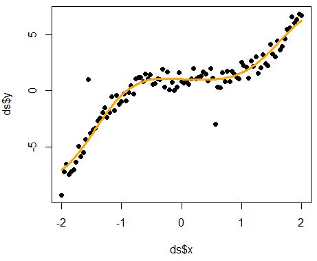
A well-designed tradeoff may be visualized in the graph below. It strikes a balance between making sufficient assumptions about the data to capture underlying patterns and avoiding excessive sensitivity to fluctuations and noises.
Conclusion
In this tutorial, we delved into the concepts of bias and variance within the context of model fitting. We offered concise explanations of bias and variance, discussing scenarios of high bias and high variance, as well as those of low bias and low variance. Additionally, we examined the intricate connection between bias and variance, known as the bias-variance tradeoff, elucidating these concepts through graphical visualizations.
The source code of the above graphs in R is listed below.
No comments:
Post a Comment